There’s 4 groups of ideas I want to disseminate from the work I’ve done thus far:
- a shared vocabulary around H-Nets
- a practitioner’s reference for empirical H-Net behavior
- better motivations for some design decisions in H-Net
- specific ’takes’ on H-Net that the paper doesn’t imply
But some of those ideas are not fully cooked, or are pending on results.
So, today’s article is a cut of the parts that I feel confident in, either context-free or with minimal results.
Primer: What are H-Nets?#
In the broadest sense, H-Nets are recursive tokenizers.
At the base of the recursion, a typical transformer-based LLM is equivalent to an $S=0$ H-Net.
If we add one level ($S=1$), we have:
- an encoder, which processes bytes
- a chunker, which compares adjacent bytes, and inserts chunk splits where pairs differ
- a main network, which selects one byte vector from each chunk as a ‘chunk vector’.
- a dechunker, which expands each chunk vector back to byte vectors
- a decoder, which improves those byte vectors to good next byte predictions
As with anything else in the byte-level modeling space, Piotr Nawrot invented this approach in 2023. The difference H-Nets make is:
- Permitting a recursive definition. $S=2,3,...$ H-Nets just imply a replacement of the main network with another H-Net itself.
- Several inductive biases that make 1D boundary learning practical in the absence of any domain-based crutches (e.g. whitespace)
Why is this desirable?#
Consider the following provocative perspective:
Why in the FUCK would you want a dynamic tokenizer??? Do you realize:
- BPE works for 99% of use cases
- BPE is cheap. A literal index lookup.
- I can’t pretokenize!!! You’re destroying infra
- transformers don’t want to see dynamic semantic bitrate!!!
Are they wrong? Mostly no. It’s important to acknowledge what a tokenizer is: a zero-FLOPs compute multiplier, practically one of the most efficient innovations in the history of text modelling.
BPE shouldn’t be challenged – it should be treated with respect.
But, even so, it should be seen as strange that, up until today, the SOTA approach used for text sequence compression in the best open source LLMs in the world remains zero-FLOPs. This is not the case in any other modality.
The widely accepted approach of Byte-Pair-Encoding is not bounded by compute constraints – it’s the exact opposite. Because the method involves zero FLOPs, it can never have the intelligence required to tokenize higher level concepts.
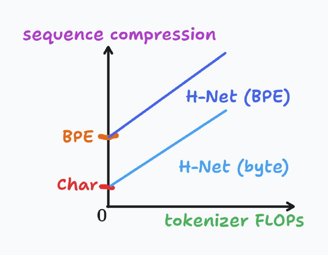
In theory, Dynamic tokenizers open a new axis of scaling – in terms of, “how much compute I want to allocate to model low-level/minute details in text”.
And, because so much research has failed to dethrone BPE, and because CALM exists, I find the following hypothesis to be most likely:
That’s not to say H-Nets are guaranteed to be a compute multiplier. I think, absent empirical evidence, you could expect either of the following to end up true:
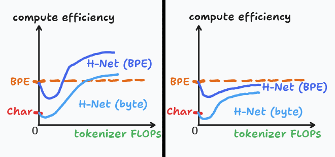
That is, even if the improved compressed tokens are a boost to the learning efficiency of the inner main network, it’s totally plausible the costs of the dynamic tokenizer still end up outweighing those gains.
So: We could live in a world where the zero-FLOPs approach is simply the most compute-optimal. Or we could live in the one where the entire LLM research community has been ignoring a gigantic compute multiplier for years on end.
Both seem a little unreasonable, you know?
So, assuming you’re on board with the premise of dynamic tokenizers.
How is a token/chunk defined?#
There are 3 competing meaningful notions of a chunk in a H-Net:
- the contiguous region of bytes which are predicted by a single chunk vector from the main net
- the exact byte vectors which are selected for consumption by the main network
- the bytes spanning from the start of a selected vector, up until (but excluding) the next selected vector
These 3 definitions map cleanly to:
- what the decoder sees
- what the main network sees
- what the encoder sees
So, in the sentence,
The encoder mixes chunks of bytes together to form useful chunk-like vectors, which are selected for processing by the main network, before being used to predict chunks of bytes in the decoder.
There is a conflation of all 3 definitions.
This is not just a gag definition. To show the importance of chunk positioning, consider the following claim:
If a H-Net decides it needs more time to think in inference, it could just choose to split chunks more often && thereby send more more tokens to the main network.
This is false under the pretraining regime, where the network can ONLY determine, in parallel, at the encoder, what chunking it assigns to the entire input sequence. You would say,
That doesn’t work! Chunking is solely determined by (3).
Interestingly, it could become less-false for a H-Net post-trained with RL, where a network could learn to control its routing autoregressively.
Case study: Spacing (fixed)#
In typical English text, you have chunks like:
[Mary ][had ][a ][little ]...[BOS][M][ ][ ][ ]...[BOS][Mary][ had][ a][ little]...
And you can intuitively see why this works: the main network always receives a space, which is responsible for carrying the prediction for the entire next word.
In text without spaces, this becomes harder, because you end up with two choices:
- Force the decoder to predict the first character of each next word without the main network’s help, which is hard.
[M][aryh][ada][l][ittle]...[BOS][M][h][a][l]...[BOS][Mary][had][a][little]...
- Force the encoder to break chunks on the last character of each word, rather than the start of the next word.
[M][ary][had][a][little]...[BOS][M][y][d][a][e]...[BOS][Mar][yha][d][alittl]...
Question: Which one do you expect to occur, empirically?
Answer
From uv run -m mh.tokens.completion:
Maryhadalittlelamb
And another example:
ThePaperFiguresShowTypicalChunksEndingInSpaces,ButCamelCaseHasNoSpaces,SoItMightBePathological
So, in both cases, it’s clearly doing the ‘hard’ strategy.
I think this is objectively a bad thing and would appreciate perspectives on the issue.
How is tokenization learned?#
The next question to ask: how do H-Nets learn to tokenize correctly?
Given a target ratio of $\frac{1}{N}$, a typical small scale $S=1$ byte-level H-Net,
- starts by randomly selecting $\frac{L_1}{L_0}$ of all byte vectors; typically $\frac{L_1}{L_0}\approx 0.4$
- quickly learns to pick almost exactly $\frac{1}{N}$ bytes, but with ~random assignment
- eventually learns reasonable chunking results, that look like words.
I call the transition $1\rightarrow2$ the ‘hockey-stick’ region, and $2\rightarrow3$ the ‘stable’ region.
Hockey-stick#
When a H-Net is implemented correctly, the compression ratio / ratio loss will
- rapidly shrink towards zero
- begin a quick spike upwards, often beyond initialization levels
- gradually taper off towards the target compression factor
And all of this happens within the first ~500 steps.
See this graph of 25 different runs (note: 1 ‘step’ is 5 optimizer steps here)
One story you could tell about how that works, is:
at initialization, cross entropy is improved fastest by short-term gains of byte statistics && simple relations like n-grams.
The predictions of the encoder+decoder are initially much more locally beneficial than the main network, which is ~noise at the start.
To reduce “noise” from the main network, selection probs shrink towards 0.
Later, the main network starts to become useful – much more useful, given that the inner transformer has much more modelling capacity than the byte-level layers – and compression factor inverts & overcompensates to push more bytes to the main network
Once those simple gains are used up, it becomes gradually easier to drive total loss improvement by reducing ratio loss towards zero, and so compression factor declines to the target.
Does that reflect the underlying reality? No, but it helps to explain some decisions and behaviors later on, so take it into account.
Signs of early disaster#
Claim: when you don’t see a quick initial hockey-stick in a H-Net run, it’s very likely your run will suck in the long run.
Consider this set of graphs:

One of the earlier experiments I did was to apply stochastic rounding to H-Net training, for memory efficiency. Although it did not work out, it provides some insight into the circumstances under which a H-Net can succeed and fail.
In the above example, the best performing curves are the ones that enter and exit the hockey-stick regime ASAP. This is quite natural, if you make the assumption that a fixed, unchanging semantic frequency over a training run is easier for a transformer to learn, than the alternative of compression ratio jumping around.
When runs don’t enter the stable regime, loss is almost always really bad.
- if ratio loss remains substantially above 1, that indicates the network wants to send an excessive number of bytes to the main network. If you know that the target compression ratio of your run is reasonable, then this indicates your network is dying.
- If ratio loss is far below 1 (lower bound $\frac{N}{2(N-1)}$), then your network is trying very hard to shut down the main network entirely, which is obviously bad
So:
Stability in the long run#
Stepping up a bit, here’s a plot of 100 runs from a compute-optimal sweep:

What lessons would you take from this? Here’s what I concluded, for some time:
Spikes in compression ratio, even in the long run, are always bad.
Vibes-based argument: transformers learn representations that make sense for a fixed bitrate of chunks. Making sequences less compressed over time is a good strategy to commit brain damage to your model, by reducing the task difficulty per vector over steps.
But after some weeks I realized that idea is wholly false. Take a look at these other set of experiments, cherry picked for “ratio exploding mid-run”:

I didn’t believe this at first, and implemented clones of the runs above with ratio loss weight cranked up:

Yet it was always true that the runs with spiking compression would outperform the ones without, in compute-equal cross-entropy.
Compression is a contest#
But if a compression ratio of 1/3 is “optimal” for the runs above, why does it take over 2000*5 steps for the above runs to reach it?
Take a look at this larger pool of runs (with varying N), and their compression ratios over time:

- compression is always by far the lowest at the lowest flops budget. In this regime, the model has very poor understanding of chunks, and is simply working to minimize ratio loss (which is always a simple task)
- With increasing compute, the inner main network is able to comprehend chunks better, and the overall network has more incentive to shrink chunk size to best fit the main network.
- With the largest compute budget, the scaling rule inverses as the main network is able to handle increasingly more compressed chunks
And in the const encoder case, I use a much larger encoder, which presumably keeps the training regime in (1) and (2), delaying the U shaped curve for much longer.

So, in short:
Extra notes on what influences compression
(I think) $p_t$’s gradient is affected by 2 things:
- ratio loss, which is a flat penalty of $(NF-\frac{N(1-F)}{N-1})/\text{seqlen}$ for selected $p_t$
- cross entropy, which contributes
- (for all $p_t$) $(2b_t-1)\langle\frac{\delta L_\text{ce}}{\delta x_\texttt{dec}},\bar z_t \rangle$, where $\bar z_t$ is output of dechunk layer
- (for select $p_t$) something like $\langle \text{EMA}^{-1}(\frac{\delta L_\text{ce}}{\delta x_\texttt{dec}}), \hat z_t-\bar z_t \rangle$, idk
(1) is “dumb” and easy to optimize for. (2) takes a long time to learn.
Conclusion#
So, what have we learned thus far?
- H-Nets are dynamic tokenizers. They’re not here to “defeat BPE”; they’re co-complementary.
- There are several ways to define H-Net chunking; clarifying it enables a clear demonstration of an interesting shortcoming of its learned boundaries.
- H-Nets have a characteristic ‘hockey-stick’ initial period of rapidly changing chunking rate,
- which happens as a consequence of the power/dumbness of ratio loss, which is weakened in the long run.
There are two other key conclusions I plan on explaining in the future:
- despite its instabilities, ratio loss is a more practical solution than static and/or loss-free alternatives
- optimal compression ratio, loss alpha, tokenizer flops, etc. ultimately has to be optimized per-domain
But they require the larger context of experimental design & other motivations, so they will be covered in a future article.