H-Net - Parameterization (Baseline)

To scale up H-Nets right on a limited compute budget, we’ll need to implement something like $\mu$transfer.

Baselines

#

If any content in the following text appears unfamiliar, please read the following materials first:

• A spectral condition for feature learning
• 高阶muP：更简明但更高明的谱条件缩放
• An Empirical Study of μP Learning Rate Transfer

My sole and only goal is to obtain a scheme which outperforms a basic Adam baseline, while permitting hparam transfer across widths.

llama+muon

#

To obtain feature learning, at init we need:

1. $||\mathbf h_\ell||_2 = \Theta(\sqrt{n_\ell})$
2. $||\mathbf W_{\ell}||_* = \Theta(\sqrt{\frac{n_\ell}{n_{\ell-1}}})$

(1) implies embedding && rmsnorm weights should be $\sigma\propto1$.

For (2), Jianlin Su says the spectral scaling’s init requirement can be approximated by $\sigma_k = \mathcal O(\sqrt{\frac{min(1,d_k/d_{k-1})}{d_{k-1}}})$, so I use that for all linear init.

We also need $||\Delta\mathbf h_\ell||_2 = \Theta(\sqrt{n_\ell})$ to be true throughout training.

• For most matrix parameters, this can be fixed with the dualizing variant of Muon, as it ensures $||\Delta\mathbf W_{\ell}||_* = \Theta(\sqrt{\frac{n_\ell}{n_{\ell-1}}})$, so long as you correctly split any fused parameters. There are two exceptions:

  • The embedding layer, which should use $\sigma=1$ && be trained with adam.

    Like any bias layer, each update will adjust its output activations by $\mathcal O(1)$ per element, regardless of the width $n$, so $\eta_\text{emb} \propto 1$

  • The lmhead layer, which folklore says to train with adam. I use η ∝ 1/d.

• For norm weights, I keep ones init && follow Lingle’s approach to set LR to 0.
• (I also use a softmax scale of $1/d_{head}$ as my scheme transfers better with it)

All of the above only ensures feature learning is width invariant. To actually empirically verify these ideas, we must

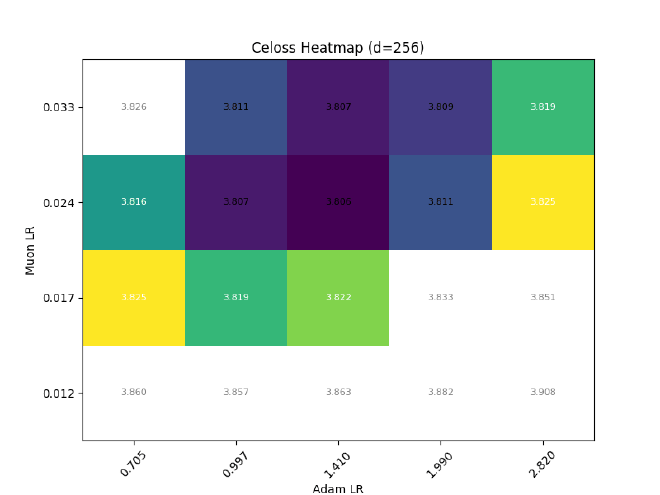
1. pick a base width/depth/mbs/steps, and sweep for its optimal base $\eta,\sigma$
2. sweep at different $d$ and check if those optimal $\eta,\sigma$ remain roughly the same

Although a proper treatment of $\mu$P would assign different layer types different constants, for simplicity I only sweep these three variables:

full_space = [
  dict(name="adam_lr", type="pow", base=2, lb=min(ADAM_LR), ub=max(ADAM_LR)),
  dict(name="muon_lr", type="pow", base=2, lb=min(MUON_LR), ub=max(MUON_LR)),
  dict(name="base_std",type="pow", base=2, lb=min(STD_RANGE), ub=max(STD_RANGE))
]
# + all runs have no wd, no grad clipping, no ema, all with WSD LR schedule,
#   betas=[.9,.95], eps=1e-6, fp32 master weights & amp bf16

The base_std constant is only applied for hidden matrices. It is not used for lmhead/emb, or for parameters that do not use normal_ init (norm weights)

After sweeping at $d=512$, I hold $\sigma$ const && grid search best LR for different $d$: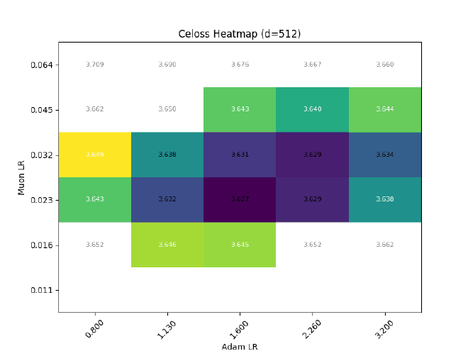

On non-parametric norms

#

Some may question the validity of keeping RMSNorm non-trainable, whether be it in pre-normalization, or within the mamba2 block, or at the end of the LM.

Here is one argument that sits well with me:

In all cases where an RMSNorm is used, its outputs are immediately fed to a linear layer. Since its affine parameters are mergable with its subsequent projections, there is no loss in expressiveness when $\gamma$ is made non-trainable.

Ofc, expressiveness != training dynamics, so I also tried training some llama2s with RMSNorm $\eta\propto1$, but (as expected) it causes optimal adam LR to quickly decrease with increasing dim: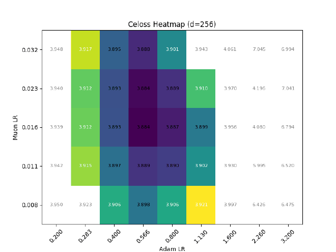

Even if I only keep the final output norm trainable, I still see divergence:

Why does this happen? In the joint $\text{linear}(\text{RMSNorm}(x))$ case, we have:

If $\gamma$ is not trainable, then $\text{RMS}(\Delta W') = \text{RMS}(\Delta W) = \mathcal O(\frac{1}{d})$ when $\eta_W\propto\frac{1}{d}, \sigma_W\propto \sqrt{\frac{1}{d}}$,

If $\gamma$ is trainable, and correlation between $\Delta \gamma$ and $\Delta W$ is small, then:

Which causes $\Delta \mathcal L$ to be dependent on $d$ and blows up $\mu$transfer.

So in theory, we could prevent this by either using $\sigma_W\propto\frac{1}{d}$ or $\eta_\gamma\propto\frac{1}{\sqrt d}$. (If you use $\eta_\gamma\propto\frac{1}{d}$, optimal muon LR decreases with width)

But this is only a solution for the final norm + lmhead, where both are trained with adam. It does not prescribe a solution for all other norm+linear cases, which involves muon (where $\sigma_W \propto \frac{1}{d}$ would be bad, and RMS would differ).

Since Lingle says non-trainable norms are OK empirically, I avoid adopting this.

Mamba2

#

There are no publicly published rules for muP+mamba2+muon. Let’s consider why.

Adam μP

#

Adam-based $\mu P$ for Mamba2 is known to work.

• This Github issue demonstrates a working coord check for a small toy mamba2 LM. Though their $\mu P$ losses are slightly worse than the SP case, it is still proof that LR transfer across widths is possible for Mamba2.
• Falcon-H1 applies the ABC-symmetry argument to shift $\mu P$ rules onto forward multipliers && init variance, while keeping $\eta$ const. Problematically, I am unable to locate the init scheme for their biases in the paper.

So, I expect the following:

• for a muon+adam $\mu P$ approach to be transferrable across widths
• for that approach to significantly outperform SP in final evaluation losses.

Easy cases

#

Some mamba parameters are easy to fit under the muP framing:

1. depthwise causal conv1d.
   • receives input xBC shaped [seqlen, d_ssm + d_state*2]
   • bias is zero-inited && $\mathcal O(1)$ updates with no LR scaling rule
   • weight is $\sigma \propto 1/\sqrt{d_{conv}}$ to be variance preserving, otherwise similar to bias
2. rmsnorm scale
   • rescales chunk scan’s out_x shaped [seqlen, d_ssm]
   • will have 0 LR & 1s init, as in transformer
3. output projection – just spectral init / msign update

Input projection

#

Mamba2’s $\texttt{in\_proj\ :}\mathbb R^{d_{model}}\rightarrow\mathbb R^{2d+2n+h}$ is an abomination. It maps the input $u$ to five different activations:

• $z_t,x_t \in \mathbb R^d$
• $B_t,C_t\in\mathbb R^n$
• $dt_t\in\mathbb R^h$ where $d = \texttt{d\_ssm}, n=\texttt{d\_state}, h=\texttt{nhead}$

If we treated each component of the projection as a separate matrix, they would get the following spectral init rules:

• $\sigma_z,\sigma_x \propto \sqrt{\frac{\texttt{expand}}{d_{model}}}$, where $\texttt{expand}=2$ by default
• $\sigma_B,\sigma_C,\sigma_{dt}\propto\sqrt{\frac{1}{d_{model}}}$

Incidentally, an STP init of $\sigma\propto\sqrt{1/d_{model}}$ would be very close to this, only differing by a constant factor of $\sqrt 2$ on $x,z$.

But, even if we do satisfy the spectral condition for each in_proj matrix, that does not imply that the downstream use of zxbcdt will retain $\mathcal O(1)$ activations.

SSM params

#

With the above init settings, mamba’s chunk scan will receive the following inputs:

• $x[T,d] \sim \mathcal N(0,1)$
• $B[T,n],C[T,n]] \sim \mathcal N(0,1)$
• $dt[T,h] \sim \mathcal N(0,1)$

and the following trainable parameters:

• $dt_{bias}[h] = \text{softplus}^{-1}(e^r)$, where $r \sim \mathcal U(ln(0.001), ln(0.1))$
• $A[h] \sim \mathcal U(-16,-1)$
• $D[h] = \mathbf 1$

which are used to compute (discretized form)

• $\Delta t = \text{softplus}(dt + dt_{bias})$
• per head $i$, where $s_{0,i} = \mathbf 0$:
  • $s_{t+1,i} = \texttt{exp}(\Delta t_i,A_i) s_{t,i}\texttt{[...,None]} + \Delta t_i x_{t,i}\texttt{[...,None]} * B_t\texttt{[None]}$
  • $y_t,i = ⟨s_{t+1,i}, C_t⟩_{\texttt{dim=-1}} + D_ix_{t,i}$

It’s (relatively) easy to see that each seq position contributes some $\Delta t\langle B_t,C_t\rangle$ factor to the output $y_t$, which implies $y$ will have coordinates $\mathcal O(\sqrt{d_{state}})$. But, $y$ is immediately rescaled after ($\texttt{out} = \text{RMSNorm}(y * \text{silu}(z)$), so $||\mathbf h||_2 = \Theta(\sqrt{d_{model}})$ is satisfied for future layers regardless.

The more pertinent issue is the LR applied to the SSM parameters. If naively interpreted as $\mu P$ adam biases, they will receive updates of $\text{RMS}(\Delta)\approx\eta$, which in the case of $A$ or $dt_{bias}$ is extremely bad, as they are both used as exponents, and will quickly exceed the reasonable representable fp32 range if $\eta$ is sufficiently high (approx $log(A)<-50$ or $dt_{bias}>100$).

This doesn’t happen in SP models, where optimal $\eta < 0.001$ even for smallish models. It also doesn’t occur in the aforementioned adam $\mu P$ baselines. For my $\mu P$ scheme, optimal base LR can even be higher than 1, so these exponents will quickly explode.

To address this, I make the incredibly unprincipled decision to lower the LRs of $dt_{bias}$ and $A$ (not $D$ as that is still $\mathcal O(1)$) by a constant factor of $2^6$. Obviously, this does not lead to steepest descent or anything otherwise well-motivated, but I do not have the intelligence to solve this issue.

So, with the above planning, do I get transferrable LR with width?

Nope.

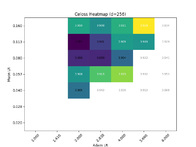
Among other problems, the Muon LR clearly experiences a strong downwards drift, from $\eta_\text{muon} \approx 0.11 \rightarrow 0.04$ ($d=256\rightarrow 2048$)

Fixing RMS

#

Based off Kimi’s assumptions, the dualizing variant of Muon should give:

So the updates to our in_proj should scale as,

• $\text{RMS}(\Delta W_{z,x})\propto\frac{1}{\sqrt{d_{model}}}$
• $\text{RMS}(\Delta W_{B,C})\propto\frac{\sqrt{d_{state}}}{d_{model}} \propto \frac{1}{d_{model}}$
• $\text{RMS}(\Delta W_{dt})\propto\frac{\sqrt h}{d_{model}} = \sqrt{\frac{\text{expand}}{d_{head}}}\frac{1}{\sqrt{d_{model}}}\propto\frac{1}{\sqrt{d_{model}}}$

In contrast, alxndrTL’s adam $\mu P$ scheme, should give:

So, I tried the two following ideas out:

1. “Since $\mu P$ adam’s RMS is lower, we should shrink $\eta_{z,x,dt}$ to scale as $\frac{1}{d_{model}}$”
2. “Maybe slow $\Delta W_{B,C}$ updates are the issue, and we can grow $\eta_{B,C}$”

(1) worked, (2) didn’t.

But even if this works, isn’t this still a bad idea? Doesn’t shrinking $\eta_{z,x,dt}$ cause feature updates to shrink towards 0 in the limit?

Perspective change

#

Actually, it is possible to argue if you consider $W_z$/$W_x$/$W_{dt}$ as concatenated head weights, rather than as whole matrices.

Consider if we decompose each $W\in\mathbb R^{d_{model},\times d_{ssm}}\rightarrow\mathbb R^{d_{model}\times h\times d_{head}}$:

• $\sigma_z,\sigma_x\propto \frac{1}{\sqrt{d_{model}}}$ (same)
• $\text{RMS}(\Delta W_{z,x})\propto\frac{\sqrt{d_{head}}}{d_{model}}\propto\frac{1}{d_{model}}$ (shrink to adjusted update)

So full param msign + rescaling $\eta_{z,x}$ by $\frac{1}{\sqrt{d_{model}}}$ gives the same $\mathcal O(\frac{1}{d_{model}})$ update RMS that head-wise muon would, which makes the $z,x$ case reasonable.

Note that:

• A similar head-splitting argument can be made for $W_{dt}\in\mathbb R^{d_{model}\times h}$.
• $\eta_{z,x}$ rescaling is necessary – muon LR still drifts if only $\eta_{dt}$ is rescaled.

Also, as a separate motivation, you might want $dt=W_{dt}x$ and $dt_{bias}$ to update at similar magnitudes to keep $\text{softplus}(dt+dt_{bias})$ stable.

TLDR

#

Initialization:

• $A_{log}, dt_{bias}$ should use mamba2’s bespoke rules
• $D$ and norm.scale should use ones init
• $W_{conv}$ has $\sigma\propto\frac{1}{\sqrt k}$, conv bias zero init
• $W_\texttt{in\_proj}$/$W_\texttt{out\_proj}$ follow spectral condition. in_proj should be interpreted as a fused split of 5 matrices: .split([d_ssm, d_ssm, d_state, d_state, self.nheads], dim=-2))

LRs:

• norm.scale non-trainable.
• Group all $A_{log}, dt_{bias}, D, W_{conv}, \texttt{conv1d.bias}$, under a param group. Downscale their LR by a reasonable factor (I settled on $2^6$) relative to lmhead/embedding adam LR
• $W_\texttt{out\_proj}$ and $W_\texttt{in\_proj}$ use muon w/ dualizing update scale, but in_proj requires either:
  • each set of 5 parameters to have LR rescaled by $[\frac{1}{\sqrt{d_{model}}}, \frac{1}{\sqrt{d_{model}}}, 1, 1, \frac{1}{\sqrt{d_{model}}}]$,
  • or interpret muon’s update rule head-wise.

All of the above claims only apply with $d_{state}$/$d_{conv}$/$d_{head}$/expand=2/ngroups=1 held const. Do not expect transfer if you modify them.

Performance

#

But do those baselines actually outperform standard paramterization in the compute optimal regime?

Well, sure:

The gain is less pronounced for mamba2:

But I assume this is because the mamba2 variant I’m using has $d_\texttt{nonssm}=0$ && no MLPs, reducing the overall gain for Muon.

Future researchers may consider testing a similar condition of ablating muon improvement on transformer vs pure attention layer stacks.

Later, I realized I had accidentally ran all of the above runs with nesterov=False in Muon.

Here is a comparison of with / without nesterov:

As you can see, there is basically no difference.

Conclusion

#

As expected, $S=0$ H-nets (which llama/mamba are instantiations of) are amenable to $\mu$transfer.

In a future article, I’ll describe my $S=1$ $\mu$P setup.