8. Length Extrapolation and Positional Robustness

In the previous article, “The Road to Transformer Upgrades: 7. Length Extrapolation and Local Attention”, we discussed the length extrapolation ability of the Transformer. The conclusion was that length extrapolation is an inconsistency problem between training and prediction, and the main idea to solve this inconsistency is to localize attention. Many improvements that exhibit good extrapolation are, in some sense, variations of local attention. While it is true that based on various metrics for language models, the local attention approach does seem to solve the length extrapolation problem, this “forced truncation” approach might not align with some readers’ aesthetics, as it feels too manually crafted and lacks naturalness. It also raises questions about their effectiveness in non-language model tasks.

In this article, we will revisit the problem of length extrapolation from the perspective of the model’s robustness to positional encodings. This approach can improve the length extrapolation performance of the Transformer with minimal modifications to the attention mechanism. It also applies to various positional encodings and is generally a more elegant and natural method, applicable to non-language model tasks as well.

Problem Analysis

#

In previous articles, we analyzed the reasons behind length extrapolation and concluded that “length extrapolation is an inconsistency problem related to length between training and prediction”. Specifically, there are two points of inconsistency:

1. Positional encodings that have not been trained are used during prediction (whether absolute or relative).
2. The number of tokens processed by the attention mechanism during prediction far exceeds the number during training.

Regarding the second point, it states that more tokens lead to more dispersed attention (or increased attention entropy), causing inconsistency between training and prediction. We have already initially discussed and solved this in “Viewing Attention’s Scale Operation from Entropy Invariance”. The solution is to change Attention from

to

where $m$ is the training length and $n$ is the prediction length. With this modification (hereinafter referred to as “$\log n$ scaled attention”), the attention entropy changes more smoothly with length, alleviating this inconsistency. My personal experimental results show that, at least in MLM tasks, “$\log n$ scaled attention” exhibits better length extrapolation performance.

Therefore, we can assume that the second point of inconsistency has been initially addressed. The next step is to focus on solving the first point of inconsistency.

Random Position

#

The first point of inconsistency is “positional encodings that have not been trained are used during prediction”. To solve this, we should ensure that “positional encodings used during prediction are also trained during the training phase”. A paper submitted to ACL22 under anonymous review, “Randomized Positional Encodings Boost Length Generalization of Transformers”, was the first to consider this problem from this perspective and proposed a solution.

The paper’s idea is very simple:

Random Position Training Let $N$ be the training length (paper uses $N=40$) and $M$ be the prediction length (paper uses $M=500$). Choose a large $L > M$ (this is a hyperparameter, paper uses $L=2048$). During the training phase, a sequence of length $N$, which originally corresponds to position sequence $[0,1,\cdots,N-2,N-1]$, is now changed to randomly selecting $N$ non-repeating integers from $\{0,1,\cdots,L-2,L-1\}$ and sorting them in ascending order to serve as the position sequence for the current sequence.

Reference code based on numpy:

def random_position_ids(N, L=2048):
    """Randomly select N non-repeating integers from [0, L) and sort them in ascending order
    """
    return np.sort(np.random.permutation(L)[:N])

During the prediction phase, positional sequences can also be sampled randomly in the same way, or points can be sampled uniformly within the interval (my personal experimental results show that uniform sampling generally works better). This solves the problem of untrained positional encodings during the prediction phase. It is easy to understand that this is a very simple training technique (hereinafter referred to as “random position training”), aiming to make the Transformer more robust to the choice of positions. However, as we will see later, it can achieve a significant improvement in length extrapolation performance. I also conducted experiments on the MLM task, and the results show that it is also effective on MLM, and the improvement is more significant when combined with “$\log n$ scaled attention” (the original paper did not include this “$\log n$ scaled attention” step).

New Benchmark

#

Many related works, including the various Local Attention and its variants mentioned in the previous article, build evaluation metrics based on language model tasks. However, whether it is unidirectional GPT or bidirectional MLM, they highly depend on local information (locality). Therefore, previous methods are likely to have good extrapolation performance simply because of the locality of language models. If we switch to a non-local task, the performance might degrade. Perhaps this is why the evaluation in this paper is not a conventional language model task, but a length generalization benchmark specifically proposed by Google last year in the paper “Neural Networks and the Chomsky Hierarchy” (hereinafter referred to as the “CHE benchmark”, which stands for “Chomsky Hierarchy Evaluation Benchmark”). This provides us with a new perspective for understanding length extrapolation.

This benchmark includes multiple tasks, divided into three levels: R (Regular), DCF (Deterministic Context-Free), and CS (Context-Sensitive). The difficulty of each level increases sequentially. The description of each task is as follows:

Even Pairs, difficulty R. Given a binary sequence, e.g., “aabba”, determine if the total number of ab and ba 2-grams is even. In this example, the 2-grams are aa, ab, bb, ba. The total number of ab and ba is 2, so the output is “yes”. This problem is also equivalent to determining if the first and last characters of the binary sequence are the same.

Modular Arithmetic (Simple), difficulty R. Calculate the value of an arithmetic expression composed of five numbers from $\{0, 1, 2, 3, 4\}$ and three operators from $\{+,-,\times\}$, and output the result modulo 5. For example, input $1 + 2 - 4$ equals $-1$, modulo 5 equals $4$, so the output is $4$.

Parity Check, difficulty R. Given a binary sequence, e.g., “aaabba”, determine if the number of b’s is even. In this example, the number of b’s is 2, so the output is “yes”.

Cycle Navigation, difficulty R. Given a ternary sequence, where each element represents $+0$, $+1$, or $-1$, output the final calculation result modulo 5, starting from 0. For example, if $0, 1, 2$ represent $+0, +1, -1$ respectively, then $010211$ represents $0 + 0 + 1 + 0 - 1 + 1 + 1 = 2$, modulo 5 output $2$.

Modular Arithmetic, difficulty DCF. Calculate the value of an arithmetic expression composed of five numbers from $\{0, 1, 2, 3, 4\}$, parentheses $(,)$, and three operators from $\{+,-,\times\}$, and output the result modulo 5. For example, input $-(1-2)\times(4-3\times(-2))$ equals $10$, modulo 5 equals $0$, so the output is $0$. Compared to the Simple version, this task includes “parentheses”, making the calculation more complex.

Reverse String, difficulty DCF. Given a binary sequence, e.g., “aabba”, output its reversed sequence. In this example, it should output “abbaa”.

Solve Equation, difficulty DCF. Given an equation composed of five numbers from $\{0, 1, 2, 3, 4\}$, parentheses $(,)$, three operators from $\{+,-,\times\}$, and an unknown variable $z$, solve for the value of $z$ such that the equation holds modulo 5. For example, $-(1-2)\times(4-z\times(-2))=0$, then $z=3$. Solving equations may seem harder, but since the equation is constructed by replacing a number in a Modular Arithmetic expression with $z$, it is guaranteed to have a solution within $\{0, 1, 2, 3, 4\}$. Therefore, theoretically, we can solve it by enumeration combined with Modular Arithmetic. Thus, its difficulty is comparable to Modular Arithmetic.

Stack Manipulation, difficulty DCF. Given a binary sequence, e.g., “abbaa”, and a sequence of stack operations composed of “POP/PUSH a/PUSH b”, e.g., “POP / PUSH a / POP”, output the final stack result. In this example, it should output “abba”.

Binary Addition, difficulty CS. Given two binary numbers, output their sum in binary representation. For example, input $10010$ and $101$, output $10111$. Note that this requires inputting the numbers at the character level rather than numerical level into the model for training and prediction, and the two numbers are provided serially rather than aligned in parallel (can be understood as inputting the string $10010+101$).

Binary Multiplication, difficulty CS. Given two binary numbers, output their product in binary representation. For example, input $100$ and $10110$, output $1011000$. Similar to Binary Addition, this requires inputting the numbers at the character level rather than numerical level into the model for training and prediction, and the two numbers are provided serially rather than aligned in parallel (can be understood as inputting the string $100\times 10110$).

Compute Sqrt, difficulty CS. Given a binary number, output the floor of its square root in binary representation. For example, input $101001$, the output is $\lfloor\sqrt{101001}\rfloor=101$. The difficulty of this is similar to Binary Multiplication, as we can at least determine the result by enumerating from $0$ to the given number combined with Binary Multiplication.

Duplicate String, difficulty CS. Given a binary sequence, e.g., “abaab”, output the sequence repeated once. This example should output “abaababaab”. This simple task appears to be of difficulty R, but it is actually CS. You can think about why.

Missing Duplicate, difficulty CS. Given a binary sequence with a missing value, e.g., “ab_aba”, and knowing that the original complete sequence is a duplicate sequence (from the previous task, Duplicate String), predict the missing value. This example should output a.

Odds First, difficulty CS. Given a binary sequence $t_1 t_2 t_3 \cdots t_n$, output $t_1 t_3 t_5 \cdots t_2 t_4 t_6 \cdots$. For example, input aaabaa will output aaaaba.

Bucket Sort, difficulty CS. Given a numerical sequence of $n$ elements (each number in the sequence is one of the given $n$ numbers), return the sequence sorted in ascending order. For example, input $421302214$ should output $011222344$.

As can be seen, these tasks share a common characteristic: their operations follow fixed simple rules, and theoretically, inputs can be of unlimited length. Thus, we can train on short sequences and then test whether the training results on short sequences can generalize to long sequences. In other words, it can serve as a very strong test benchmark for length extrapolation.

Experimental Results

#

First, let’s present the experimental results from the original paper “Neural Networks and the Chomsky Hierarchy”. It compared the performance of several RNN and Transformer models (the evaluation metric is the average accuracy of strings, not the overall perfect match rate):

The results might be surprising. The “currently popular” Transformer has the worst length extrapolation performance (different positional encodings were tested for the Transformer here, and the best value was taken for each task). The best performer is Tape-RNN. The paper gives them the following ratings:

The random position training method proposed in “Randomized Positional Encodings Boost Length Generalization of Transformers” discussed earlier, however, recovered some disadvantages for the Transformer:

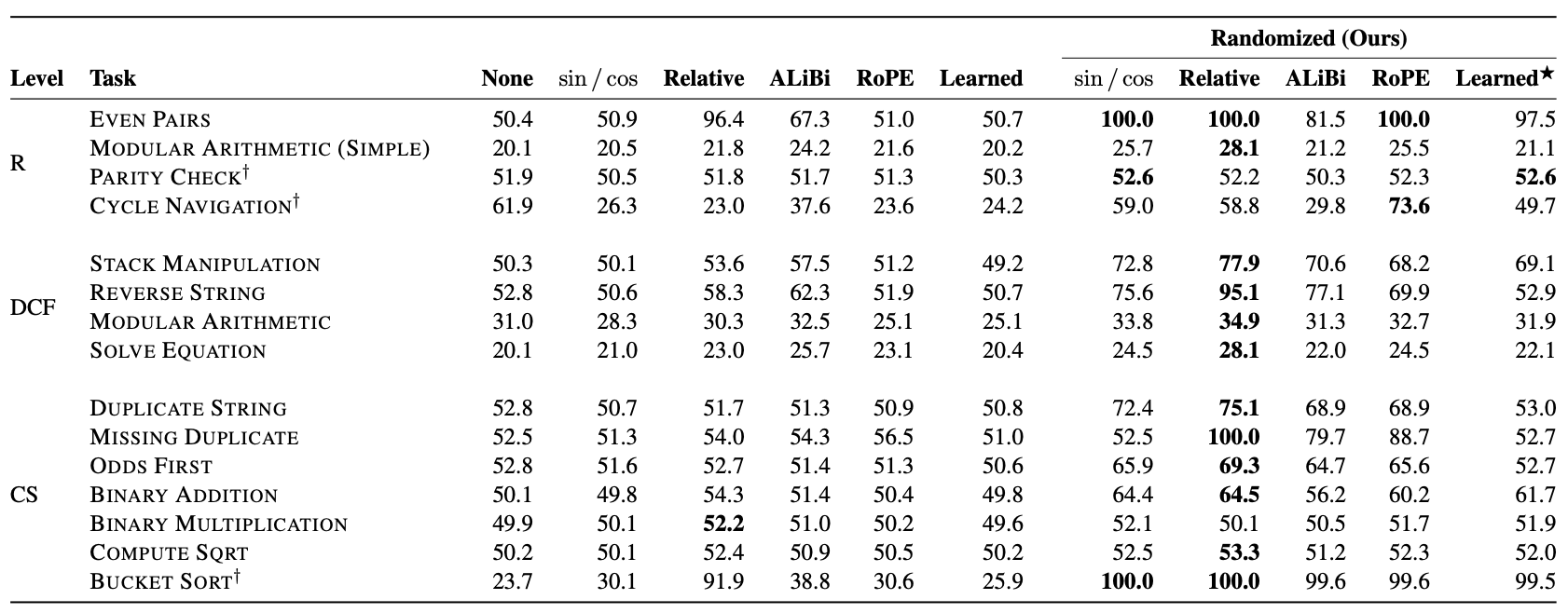
As can be seen, with random position training, the Transformer shows significant improvement regardless of the positional encoding used. This further validates the conclusion from the previous article, which is that length extrapolation performance is not strongly related to the design of the positional encoding itself. Specifically, random position training achieved perfect accuracy on the Bucket Sort task for the first time. Although the overall performance is still not outstanding, it is a significant step forward compared to previous results (wonder if combining with “$\log n$ scaled attention” could lead to further improvement?). Another point worth noting is that the table above shows that ALIBI, which performs well in language model tasks, does not exhibit significant advantages on the CHE benchmark, especially after adding random position training, its average metric is worse than RoPE. This initially confirms the previous conjecture that the good performance of various Local Attention variants is highly likely due to the severe locality inherent in language model evaluation tasks. For the non-local CHE benchmark, these methods do not have an advantage.

Principle Reflection

#

Upon deeper thought, “random position training” can be quite confusing. For simplicity, let’s assume $L=2048, N=64, M=512$. In this case, the average positional sequence used during training is roughly $[0, 32, 64, \cdots, 2016]$, and the average positional sequence used during prediction is $[0, 4, 8, \cdots, 2044]$. The difference between adjacent positions is not the same during the training phase and the prediction phase, which can also be considered a type of inconsistency. However, it still performs well. Why is this?

We can understand it from the perspective of “order”. Since the position IDs are randomly sampled during the training phase, the difference between adjacent positions is also random. Therefore, whether using relative or absolute positions, the model is unlikely to obtain positional information through precise position IDs. Instead, it receives a fuzzy positional signal. More precisely, it encodes position through the “order” of the positional sequence rather than the position ID itself. For example, positional sequences [1,3,5] and [2,4,8] are equivalent because they are both sequences sorted in ascending order. Random position training “forces” the model to learn an equivalence class, where all positional sequences sorted in ascending order are equivalent and can be interchanged. This is the true meaning of positional robustness.

However, my own experimental results on MLM show that learning this “equivalence class” is still somewhat difficult for the model. A more ideal method is to still use random positions during the training phase so that the positional encodings used during the prediction phase are also trained, but the initial part of the positional sequence during the prediction phase should be consistent with the average result of random positions. Taking the same example, if the positional sequence used during prediction is $[0, 4, 8, \cdots, 2044]$, then we hope the average result of random positions during the training phase is $[0, 4, 8, \cdots, 252]$ (i.e., the first $N$ elements of the sequence $[0, 4, 8, \cdots, 2044]$), rather than $[0, 32, 64, \cdots, 2016]$. This way, the consistency between training and prediction is tighter.

Further Extension

#

Thus, I considered the following idea:

Equal-mean Random Position Training Let $n$ follow a distribution with a mean of $N$ and a sampling space of $[0, \infty)$. During the training phase, randomly sample an $n$, and then sample $N$ points uniformly from $[0, n]$ to serve as the positional sequence.

Reference code:

def random_position_ids(N):
    """First randomly sample n, then sample N points uniformly from [0, n]
    """
    n = sample_from_xxx()
    return np.linspace(0, 1, N) * n

Note that the positional sequences sampled this way are floating-point numbers, so they are not suitable for discrete trained positional encodings, only for functional positional encodings such as Sinusoidal or RoPE. Below, let’s assume only functional positional encodings are considered.

The biggest problem with this idea is how to choose a suitable sampling distribution. My first thought was the Poisson distribution, but considering that the mean and variance of the Poisson distribution are both $n$, then according to the “3$\sigma$ rule” estimation, it can only extrapolate to a length of $n+3\sqrt{n}$, which is obviously too short. After selection and testing, I found that two distributions are more suitable: one is the Exponential distribution, whose mean and standard deviation are both $n$. Even according to the “3$\sigma$ rule”, it can extrapolate to a length of $4n$, which is a more ideal range (actually even longer); the other is the beta distribution, which is defined on $[0,1]$. We can set the test length as 1, so the training length is $N/M \in (0,1)$. The beta distribution has two parameters $\alpha, \beta$, where the mean is $\frac{\alpha}{\alpha+\beta}$. By ensuring the mean equals $N/M$, we have additional degrees of freedom to control the probability around 1, which is suitable for scenarios where further extrapolation range is desired.

My experimental results show that “equal-mean random position training” combined with “$\log n$ scaled attention” achieves the best extrapolation performance on the MLM task (training length 64, test length 512, sampling distribution is Exponential distribution). Since I haven’t worked on the CHE benchmark before, I couldn’t test the effect on the CHE benchmark for now and will have to leave it for later opportunities.

Summary (formatted)

#

This article analyzed the length extrapolation of the Transformer from the perspective of positional robustness and proposed new methods like “random position training” to enhance length extrapolation. At the same time, we introduced the new “CHE benchmark”, which has stronger non-locality compared to conventional language model tasks and can more effectively evaluate work related to length extrapolation. Under this benchmark, previous attention localization methods did not perform particularly outstandingly. In contrast, “random position training” showed better performance. This reminds us that we should evaluate the effectiveness of related methods on more comprehensive tasks, not just limited to language model tasks.

@online{kexuefm-9444,
        title={The Road to Transformer Upgrades: 8. Length Extrapolation and Positional Robustness},
        author={苏剑林},
        year={2023},
        month={01},
        url={\url{https://kexue.fm/archives/9444}},
}